OpenOffice 3: Calc
by Meemaw
We have looked at OpenOffice Writer, covering some of the basics of the program and what was included. This month we'll look at some of the basics of OpenOffice Calc, which is the spreadsheet program in the OpenOffice suite. When you open it, you will have an empty spreadsheet grid for whatever data you want to organize. This will be a very basic review, because there are many things that Calc can do that I've never used.
The toolbars are almost identical to those found in OO Writer; however, some of the individual buttons are different. The main toolbar has all the standard features, like cut & paste, save, open, new , print, etc. The formatting toolbar is different in places. Instead of the numbering and bullet buttons that are used in Writer, you will have buttons for changing cell contents. You can highlight cells and format them as currency, add or subtract a decimal place from your numbers or put borders around specific cells. Instead of editing text, you can choose a filler color for the cells you have highlighted. Also, two sorting buttons are in the top row to sort your data alphabetically, or reverse. You can also display a graph to go with your data if appropriate.

Spreadsheets can be used for quite a few projects! In addition to keeping track of monetary amounts for each month of the year (only one use), you can build forms (like invoices or statements), make address lists (you can do this in a database program, but if you only need name, address, city & state, a spreadsheet is just as easy, if not easier.) I use spreadsheets to do address labels quite often.
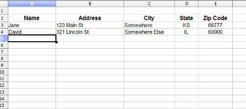
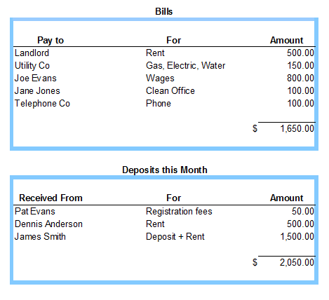
In my job, I have to submit a list of upcoming bills to my bosses, so they know where the money is being spent each month. I use a spreadsheet because you can set it to add a column of figures. That way, they know the total, and I don't have to run an external adding machine three times to make sure I didn't add wrong!!! In the example, I did a quick home budget list that is similar.
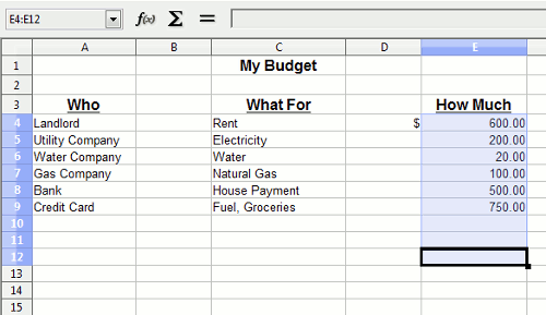
In the next shot I highlighted the numbers in the money column, starting with the cell where the sum should be displayed and dragging my mouse up. Then up above the spreadsheet (but below the toolbars) in the formula bar, click on the symbol (Σ). Your sum should appear in the bottom cell.
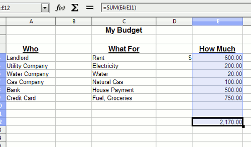
The formula bar has the characters that are in the cell you have selected. If you have numbers or text in the cell, the formula bar will show what is there. If you are doing a spreadsheet with mathematical calculations in it (like the number sum above), it will show the formula for getting that answer. In the example above, the formula is =SUM(E4:E11) which means that the numbers in cells E4 through E11 will be added together and the answer displayed in E12 (which is the cell where the formula is located.) In a budget, for example, we could add our income and bills separately, then put a formula in a third cell which would stand for the difference between incoming and outgoing cash to let us know our month-end balance. The Insert > Function menu has a list of formulas you can use. You can also get the same list from the fn button to the left of the formula bar.
You can make your document a little prettier, if you wish, by putting colored backgrounds in some of the cells. I highlighted 5 cells, then clicked on the background color button on the toolbar, and chose a light blue. I also made the row height smaller, so that my cells would look like a colored border. Click on Format > Rows > Row Height (or Format > Column > Column Width) to change the size of the row or column - or if your hands are very steady, you can 'grab' the row border at the bottom of the box with the row number in it, or the column border at the right of the letter, and drag it to suit you. You can get close, but if you want several of them the same width or height, you're more accurate highlighting the ones you want to change and using the format menu.
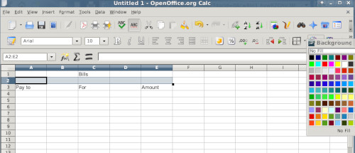
You can go through and color cells and put your information in until you have it the way you want it. You can always click the 'Print Preview' button to see what it looks like (and with a little more than 15 minutes work, I'm sure you can make one that's awesome!)
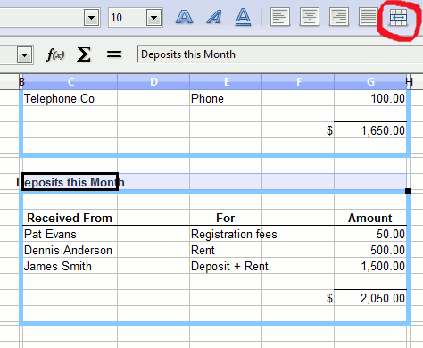
Another thing you can do that might make your spreadsheet look a little better is to merge cells. Sometimes I'm doing a sheet that needs a title, and I want the title centered. If the title is in the spreadsheet itself, I highlight the number of cells that equal the width of the sheet, then click the 'Merge Cells' button.
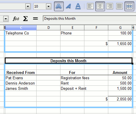
If you haven't clicked on the 'Center Text' button, do that as well. In some of the spreadsheets I do, the columns are different widths, so merging the cells and centering the text gets it centered the way I want it.
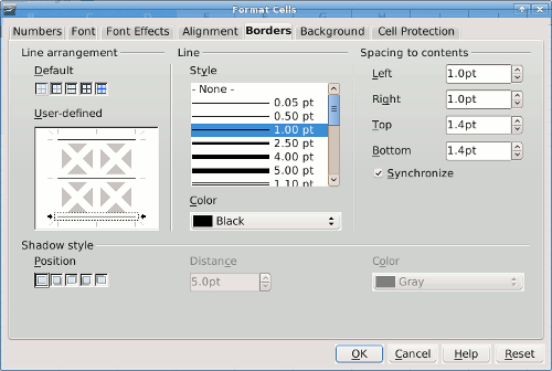
You can format the cells to add lines in specific places (like underneath the headings in each section or at the bottom of a column of numbers being added) or have your numbers show in a particular format. Just highlight the desired cells and click Format > Cells and you'll get a formatting box; use the arrangement section at left to designate the locations of the lines and the style box to make the line the correct thickness. I actually changed mine to 2.50 pt.
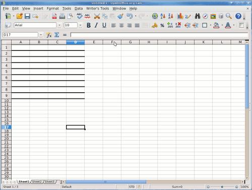
If you only have a few places you want the borders to go, you can highlight the cells and use the Borders button on the toolbar (in my example, the borders button is in the bottom row of tools to the left of the background color button). You will get a drop down with several choices.
In the same formatting box, the tabs across the top include 'Number.' This is where you can format numbers to look the way you want them. In a financial worksheet, I like them all to have two decimal points and a comma for the thousands place. I format them as numbers rather than currency. Why? Because when you format them as currency, each number includes the currency label you choose, and I only want my dollar signs at the top and bottom of each series, not on every amount. Therefore, I use an extra column to the left of my numbers so I can put the dollar signs where I want them.
Now, if you've gone to print your spreadsheet, and it says 'Sheet 1' at the top — and you don't know who put it there — you should go to Format > Page and choose the 'Header' tab. There is a button that says 'Edit.' Click that one and you will see a chart showing items displayed in the header of your document. The center section has 'Sheet 1'. You can delete that text, or you can cancel out of that, go back to the header tab and uncheck the 'Header On' box. Conveniently, there's usually more than one way to do something.
Just like in Writer, OpenOffice.org has loads of templates for use in Calc. You can find templates for graph paper, budget sheets, amortization schedules, grocery lists and even a Sudoku game!
There are exterior sites that have templates as well. If you are looking for a specific template, you can go to one of these sites:
I've found loan payment schedules, budget sheets, the Sudoku game and even graph paper! Even though many of them say Excel, we know we can open them anyway.
Calc will do much more than what is covered here! I hope you'll take some time to explore. Next time, we'll look at Impress.


