
| Previous
Page |
PCLinuxOS
Magazine |
PCLinuxOS |
Article List |
Disclaimer |
Next Page |
LibreOffice Tips & Tricks, Part 3
|
|
by Meemaw In this third installment of our series, we will look at LibreOffice Calc, and ways to spice up your spreadsheet, protect your hard work and make some of it a bit easier. Autoformat Tables Some of you design your spreadsheets to be used in meetings or somewhere that people can see your handiwork. It makes sense that you don't want all your spreadsheets drab and colorless, and you also want to make certain fields stand out, like your headings and section names. You can do this by changing the background color of those cells. You can go into your table and highlight part of a row and change it, then highlight another partial row and change that, but try this first. Highlight the table you are working with, then click Format > Autoformat. A window will pop up with several choices to select, and as you go through the list, each design is displayed on your spreadsheet/table, showing you what it will look like. One of those may work for you. 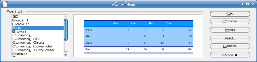 Protect Your Document Just like document protection in your Writer documents, you can password protect your spreadsheets as well. Just go to Tools > Protect Document > Sheet or Document. There you can establish password and parameters for your protection. Vary Your Charts You can always do the standard bar graph, but sometimes change to a 3D Pie Chart. Highlight the items you want in your chart, then Insert > Chart. You will get a window where you can designate your design, and a sample will appear on your spreadsheet. 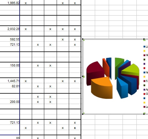 Change Status Bar Values While you are working with your sheet, click on a column of numbers, then look at the status bar across the bottom of your window. Mine says “Sum=8,482.18” which is the sum of the numbers in the column. 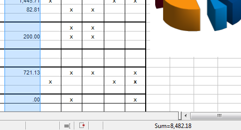 That's great for some things, but what if you want an average of the numbers? or have loads of them and want to know the largest or smallest one? Right-click your status bar there and choose what value you want to see. My chart is an expense chart. What if I want the average of all expenses? Right-click.... choose Average... and there it is. Very useful! 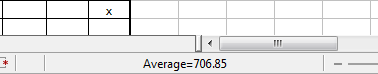 Navigator We looked at the Navigator in a text document and found it useful. Yes, you can use the Navigator in a spreadsheet as well. If your spreadsheet is large, or has several sheets, the Navigator should help you get around in it pretty quickly. The Navigator lists sheet names, links, graphics, conditional formatting, values and a few other items. Functions Suppose you have an expense sheet that you just constructed. How do you total your expenses? You can highlight the column, look at your status bar and see what the sum of your numbers is. You can also add it up on the calculator and type it in. However, this is a spreadsheet and those kinds of functions are built-in. One way is to click on Insert -> Functions. A window will pop up asking what kind of function you want to insert. This is good when you are constructing your sheet but haven't entered all your values yet. The Function window contains all the functions programmed into Calc. You can choose the one you need and enter the cells you want to use. 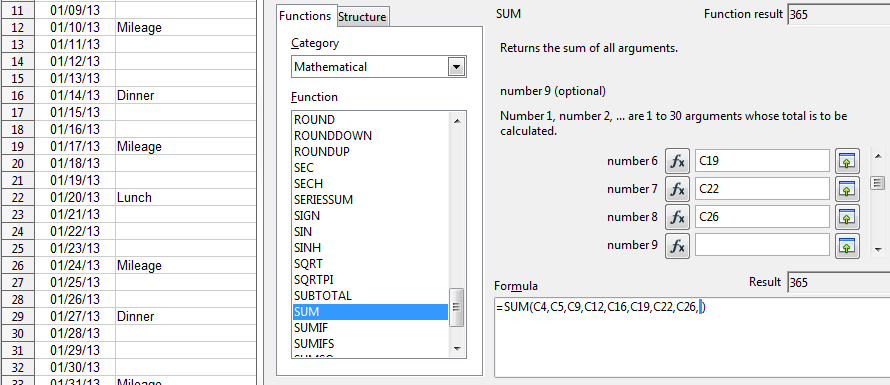 I want the sum of all the expenses for January. As you can see, I only entered the cells that actually have numbers in them. While this works many times, it is a little tedious. When I'm doing a budget and only want to add certain lines together, I can use this method. If the column is a line of cells that can all be added, there is a faster way. Starting with the cell where you want your sum, click and highlight the whole column clear up to the first cell that could be used. Now, click the sum symbol to the left of your input line, and your formula will appear. Notice that instead of each filled cell being listed, you have a range of cells to be included in that sum. I actually use both methods on my budget. 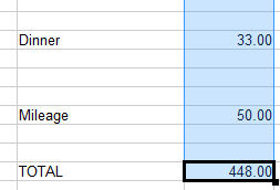 You can copy that design onto a different sheet (for February maybe?) and do the same thing. The good thing is that if different cells in that range are filled, you will still get a sum at the bottom. You want to check to make sure you have the correct range in your input line for that cell. My boss asks me to make a report of bills that need to be paid every month. I use the same spreadsheet every month and have the column set up to add the amounts together. It's always correct, and all I have to do is change the names, descriptions and amounts every month. Change the Function of the Enter Key It's possible to change the function of the enter key. By default, when the Enter key is pressed, the cell below the current working cell is selected. However, if you need to keep moving right frequently, you can set the function of the enter key to move to the immediate right side cell, each time the Enter key is pressed. This is located in Tools > Options > LibreOffice Calc > General. Auto-Fill I am wanting to make a schedule for employees who work for me. Rather than using one of the calendar templates, I am going to list the days of the month in a spreadsheet and list the employees who work on each day. Numbering is really tedious, though so I will do it differently. After I set up my title and headings, I will enter a 1 in my ‘Date' column. Then, moving my mouse to the bottom right corner of that cell until my mouse pointer changes to a plus sign, I click and drag down my column until I have highlighted 31 spaces (I'm doing October's schedule). When I lift my finger off the mouse, the column will be numbered. Quick and neat! I did have to leave that cell and then click back into it before I got the plus sign. Also, if you don't get enough cells filled to suit your needs, click on the last cell filled and repeat the process, and auto-fill will continue on with the number sequence. If your sequence is to be different, like 3, 6, 9, and so on, just put the first two or three numbers in, highlight all the cells you just filled and do the same. Auto-fill will finish it for you. It works with dates, too! 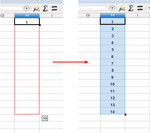 Freeze Columns If your spreadsheet contains a lot of columns, certain columns can be frozen on the screen while the remaining columns move freely. For example, if your first two columns are Name and Company, these two columns can be frozen on the left hand side of the chart while viewing the data in the other columns. Highlight the column to the right of the ones you want to freeze, then click on Window > Freeze. Everything to the left of the column chosen will be in the ‘freeze zone'. Freezing them will enable you to be able to tell which Name & Company each piece of your data belongs to. In the example below, I chose one cell, to the right of the series of dates in my employee schedule, and below the headings. This keeps the dates and the headings visible as I scroll through the sheet.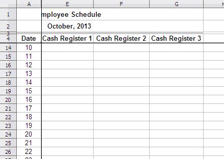 Text Formatting If you enter a number like 00643 in a cell, it automatically becomes 643 due to the default formatting. You can always right click and format the cell as text, but you can also you could just enter '00643 and the cell is automatically formatted as text and the value is entered as it is. This can also be applied to text, dates, etc. However, you cannot apply formulas to such cells. Auto-Filter One of the spreadsheets I use often includes mostly names and addresses. There are hundreds of entries on this particular sheet. I may want to check the names of the members who live in ‘Colorado'. I can highlight the ‘State' column and apply the auto-filter (Data > Filter > Auto-Filter) to this particular column. A drop box appears on the top of the column. It will have the states contained in this column, and I can select ‘Colorado' from the drop box to see only the rows with a value of ‘Colorado' in the ‘State' column. Cool, huh? 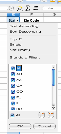 If you decide you don't want or need this filter any longer, you can go back to the same menu location and uncheck Auto-Filter. Amazingly enough, many of the items in this article were things I didn't know, and have just learned from my research! Many of them have made my work much easier. Next month we will look at LibreOffice Impress to see how we can speed up the creation of a presentation. |